Introduction
Math seems to be a scary thing for many people. If you tend to get scared by thinking about numbers and what to do with them, this module is for you. We will tame the beast and show you how much you can do – with counting, adding, and dividing numbers.
Common problems we address
When working with data, we run into a few common problems we will address with the methods we learn here:
- What is “normal”?
- What is different / special?
- How do I compare two different entities (e.g. countries)?.
What am I dealing with?
When working with multiple values in data, one of the key points of information you can get is how the data is distributed. This helps you figure out what you are dealing with.
Range
The first thing you want to look at is the range of your data: from where to where does your data stretch? Does it start with small numbers? Large numbers? Does it run from negative to positive? All this is essential information that will help you to deal with your data.
Looking at the range will also help you to find errors in your data. Let’s say you are comparing body heights and that you’ve asked people to enter their size in centimetres. Say you find that your data’s values range from 127 to 622. There is clearly a mistake: 6m tall people are very rare, and the likelihood for you to have caught one is relatively small. You should go back to your data and check it.
What do you have to do to find your range? Simply go through your data and find the minimum and maximum value—the lowest and the highest, respectively. In a spreadsheet, you can do this with the formulas =MIN and =MAX.
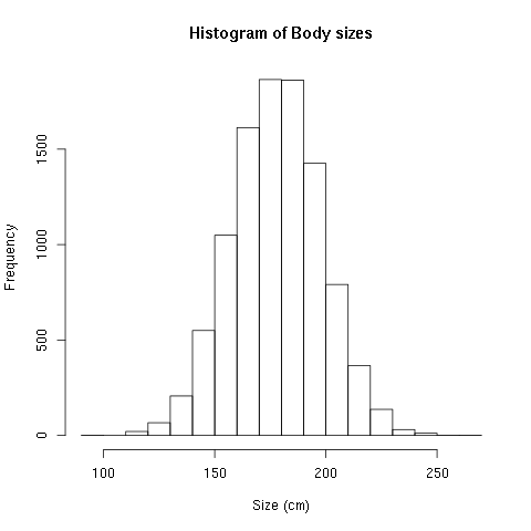
Let’s say you have the following data (let’s take body sizes):
163.1 162.2 210.5 201.0 188.7 182.6 153.0 173.5 146.6 148.0
Question: What is the range of your dataset?
Hint: find the lowest number (minimum) and the highest number (maximum).
Answer: Our range is from: 146.6 to 210.5
How many do we have?
The next important question we can ask ourselves is: how many things do we have? e.g. how many people did we survey? How many countries do we know things of? etc. This might seem simple, but for statistics, this is very important.
How do we get it? Simply count! In spreadsheets, this would be the formula =COUNT or =COUNTA.
In the data below: How many data points do we have?
163.1 162.2 210.5 201.0 188.7 182.6 153.0 173.5 146.6 148.0
10! Easy, isn’t it? Simply by counting and looking at our range, we already have valuable information! Let’s look at more.
Distribution
Next you want to look at is how the data is distributed. This is commonly done with a plot called a histogram. A histogram simply counts how often each value appears and proceeds from there.
So how do we do this? This is commonly done by binning data. What does this mean? Basically, we create bins, which are the ranges of numbers we care about.
Let’s do this for the data we used above. Our data ranges from 146.6 to 210.5—let’s create reasonable bins. Let’s say we use 140-160, 160-180, 180-200, and 200-210. Then we go on and—surprise—count. How many values do we have between 140 and 160? How many between 160-180? And so on.
Result:
| Bin | Number |
| 140-160 | 3 |
| 160-180 | 3 |
| 180-200 | 2 |
| 200-220 | 2 |
Fantastic- let’s draw this as a simple graphic:
140-160: ***
160-180: ***
180-200: **
200-220: **
This is all there is to histograms, which show us how our data is distributed.
While this doesn’t tell us much if we have only ten values, this is super useful if we have more.
Things we want to look at: how many peaks do we see? Is there a single or multiple peaks? (Multiple peaks can tell us something about different groups present.) Is this a normal distribution where there is a clear peak and the sides are equally distributed (as below)?
Or is the distribution “skewed” (i.e. there is a peak on the left and a long tail to the right)?
The distribution tells you what kind of further descriptors are practical to use.
What is Normal?
One of the next questions often is: what is “normal”? What we mean by this is: how can I tell whether something is worth looking at? (We’ll figure out what is special further below.)
There are different ways to find this out.
Mean
The mean (or “average”) is the most commonly used way of looking at what is “normal”. We know it from newspaper articles claiming that the “average income” is increasing or decreasing and so on. But how do we calculate it? Quite simple: we sum up all the numbers we have and divide the result by the number of numbers we have.
For example, the mean of 1, 2, 3, 4 = (1+2+3+4)/4 = 10/4 = 2.5.
Can you calculate the average of the heights we used before?
163.1 162.2 210.5 201.0 188.7 182.6 153.0 173.5 146.6 148.0
Answer: the mean is 172.92.
The mean is a great tool if your data is normally distributed. In that case, it tells you quite a bit about where the maximum of the distribution is and thus what you would perceive as normal.
Median
Let’s look at a different example. If we look at income distribution in countries, the distribution is not normal. It rather looks something like:
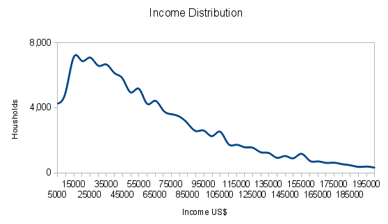
Now, if you look at the mean income, that might be quite a number. But if you earn less than the mean, you could still earn more than half of the population simply because the majority of the population earns so little. The median tells us this. To calculate the median, we simply sort the data we have and pick the value right in the middle.
Let’s calculate the median of the following data:
162.0 159.1 169.9 191.3 195.9 139.8 186.0
First we’ll sort the data (ascending or descending does not matter)
139.8 159.1 162.0 169.9 186.0 191.3 195.9
Then we’ll pick the value right in the middle: 169.9 – this is our median!
What if we have an even number of values? We simply take the mean of the two values right in the middle.
Can you calculate the median of:
163.1 162.2 210.5 201.0 188.7 182.6 153.0 173.5 146.6 148.0 ?
Result: 168.3, the average of 163.1 and 173.5
Mode
Sometimes neither the mean or the median really tell us what we want to know. Let’s look at a survey where we asked people how many siblings they have. They responded:
0, 1, 1, 1, 1, 2, 2, 2, 3, 5
well have a mean of 1.8 siblings, a median of 1.5 siblings. But what we really want to know is: How many siblings do the most people say they have. So we start counting.
0 - 1
1 - 4
2 - 3
3 - 1
5 - 1
We see 1 is the most frequent answer. This is the mode.
What do we do if the data is not discrete? We create bins as we did above, then count.
Sometimes you will not end up with a clear winner. There might be two different values that get the same number of counts. In case they are clearly separate, we call this a bi-modal distribution (or multi-modal in case it’s more than two).
How big is the variation in the data?
The next thing we want to know is how big the variation is in our data. Two measures come in handy: the standard deviation and the median absolute deviation. The standard deviation comes with the mean and is very frequently used. The median absolute deviation is less well known and would be the best to use if you’re using the median already.
Standard Deviation
So let’s look at the first thing, the standard deviation. It tells us how much, on average, data points are off the mean. We calculate it by summing up the square of the differences of the values and the mean, then dividing that sum by the number of measurements minus one, then taking the square root of that—did you even pay attention?
More importantly: If we do have a normal distribution – 68.27 percent of data points will fall within one standard deviation from the mean and 95.45 percent within 2 standard deviations from the mean. So it gives us a good idea where most of our data is. Hard to remember- this illustration shows it pretty clearly:
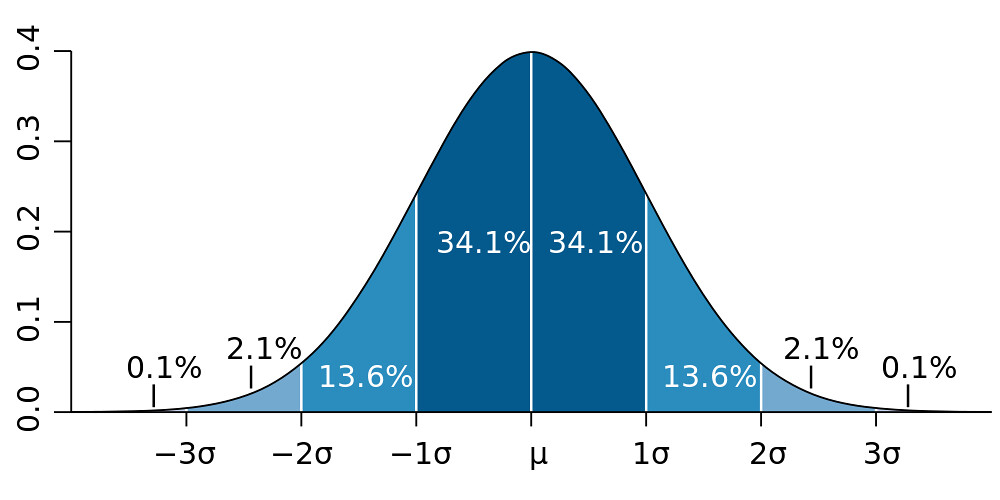
Image CC-by Wikipedia Member Mwtoews
Sounds complicated; let’s do it.
Let’s take our data above: 1, 2, 3, 4.
We already know the mean is 2.5.
Let’s calculate the standard deviation:
| Value | Difference to mean | Squared Difference |
| 1 | -1.5 | 2.25 |
| 2 | -0.5 | 0.25 |
| 3 | 0.5 | 0.25 |
| 4 | 1.5 | 2.25 |
So we’ll sum up the squared differences: that’s 5.
We’ll divide 5 by our number of data points minus 1.
5/(4-1)
That’s 5/3.
And now we’ll take the square root of that.
And we arrive at 1.291. – this means that 68.27% of measures will fall in this distance from the mean (assuming we do have a normal distribution).
Sounds complicated! It is a little. But remember, it’s just adding stuff up, multiplying, and dividing. No big magic here. Luckily, if you need it, spreadsheets have a formula for this: =STDEV.
Median Absolute Deviation
As we said, the standard deviation works well when you can use the mean, since it’s based on the mean. But what about when you use the median? Use the median absolute deviation. It works very similarly, but it’s
easier: you calculate your median and the absolute difference between each value and the median. Then you calculate the median of the differences.
For example: our data is
1, 2, 3, 4, 5
The median is 3.
The differences are: 2 1 0 1 2 – sorted, 0 1 1 2 2.
The median absolute deviation is: 1.
Sounds feasible,
right?
Normalizing Data – aka. comparing things
Once we have an idea of what we’re talking about, let’s figure out how we compare things.
Let’s say we want to compare two countries that are quite different in several aspects. If we want to compare their GDPs, for example, we can do so, but it will not tell us anything useful. If, for example, one country is very big and another is very small, the bigger will have the higher GDP. Does that mean it’s more productive? No. We’ll have to compare them on equal footing. Usually this is done using something that tells us how big a country is; in countries, that’s often population.
To compare productivity, we can divide the GDP by the population. This is called normalization. Now we can compare the GDP per capita. This is so commonly done that you will probably have heard of this indicator.
Another way of normalizing values is to use percentages. For example, if you want to compare what countries spend on health, it is great to normalize this by the GDP (e.g. to say this country spends a relatively great amount on health, whereas this other country doesn’t). Or think of
elections: we commonly encounter percentages there (e.g. we calculate how many people voted for party A and divide this by the number of valid votes).
Finding out what’s special – Z-Scores
Z or standard scores are a good way to figure out what is special. Let’s say you have election results and want to find places that are interesting to report on. One thing you can do is figure out where a party has done exceptionally well. Z-Scores are great for this.
The Z-Score of a measurement is calculated as
(x – mean)/standard deviation.
The Z-Score gives you a value’s distance in standard deviations from the mean. You can now set arbitrary limits and say: places where the votes with a Z-score higher than 2 are interesting because this means that extraordinarily many people voted for a specific party. A Z-score below -2 is also interesting because exceptionally few people voted. You can make this a little finer by looking at Z-scores for counties or regions (often there are regional differences and so on). Remember – 95.45 percent of measures fall into 2 standard deviations from the mean (if you have normally distrubuted data) this means: there is less than a 5 percent change for the Z score to be higher (or lower) than 2. 5% makes you pretty stand out. Not enough: 3 Standard deviations give you less than 1% of chance (99.73% of points are within 3 standard deviations from the mean in a normal distribution).
Overall, the Z-Score is a handy addition to your toolbox for figuring out what data values are different.
Recap
In this module, we talked about the basic math you need to understand quantitative data. We talked about how to figure out what you are dealing with (this is commonly called descriptive statistics). We went
on to figure out how we could compare apples to oranges (if we wanted to), and finally we looked at Z-Scores to be able to figure out what is special about something.