Advanced Spreadsheet Formulas

Module objectives

• Discover advanced uses of formulas

• Learn Vlookup for joining sheets

Module requirements

Having followed the first part of the Getting Smart with Spreadsheets module.

And the following:

• A google docs account

• The spreadsheet with education budgets for local councils in Tanzania – create a working copy!

Table of contents

• Introduction

• Advanced Formulas

• Joining Sheets

• Extension activities: Queries

Introduction

Let’s continue our journey into spreadsheets. If you already know how to use basic formulas and make use of pivot table wizards, you’re already in a great shape for working with data. But sometimes, you need to be able to work with the data more directly.

In this tutorial, you’ll learn how to make use of rather more complex formulae, including how to join data from multiple spreadsheets into a single sheet sheet as well as how to run database like queries over the data contained in a single spreadsheet.

Advanced Formulas

The spreadsheet we’ll be working on contains the education budgets for local councils in Tanzania (in Tanzanian shillings) and information from the census about the population living there. We want to bring the two sheets together to create a single source of information that will allow us to look at how much money is spent per-person in each region and then compare these numbers to see whether there are any noticeable regional differences.

If you inspect both of the sheets in the example spreadsheet file, you should notice that the names for the councils are presented in slightly different ways, although we shall presume that they refer to exactly the same areas. The budget sheet has a single column that contains both the name of a council as well as the region is it based in, such as “Arusha MC, Arusha”. The census sheet has two columns, one describing the region, and the other the council name. But the differences do not end there: the same location may also be given slightly different names: the census location “Arusha City”, for example, rather than the budget labelled “Arusha City”. (We need to take care when areas named in slightly different but we assume them to cover the same area: they may actually refer to slightly different regions on the ground. In an ideal world, data sets would include unique and unambiguous identifiers so that we know exactly what each data element refers to and that the data in one sheet referring to location XYZ123 is referring to the same place identified as XYZ123 in another sheet.)

Assuming that we can reliably and unambiguously map from the names in one sheet to the names in another, we need to work out a method that allows us to do this. We could do it by had, but it might take a long time – and be subject to all sorts of human error – if the dataset is large one. Instead, we’ll try to automate the process by using a combination of formulas.

If you’ve ever calculated the sum of values in a column using SUM() or found the average (mean, or median) values, you’ve used a formula. But did you know you can combine formulas, by feeding the result of one formula into another? We’ll do this in the next walkthrough.

Walkthrough: Advanced Formulas

• Within the example spreadsheet, compare the council names in the first and second sheets – try to spot any similarites and differences between them. Do any of the differences appear to be regular, or systematic?

• Notice how the budget sheet uses “MC” where the census sheet uses “City”, the same for “TC” and “Town”

• We could go through and change those manually, but let’s use a formula to do this.

• We’ll need to combine formulas in order to replace both “MC” and “TC” but first we’ll need a new column in the sheet

• Click on the small triangle next to the column letter and select “insert 1 right”

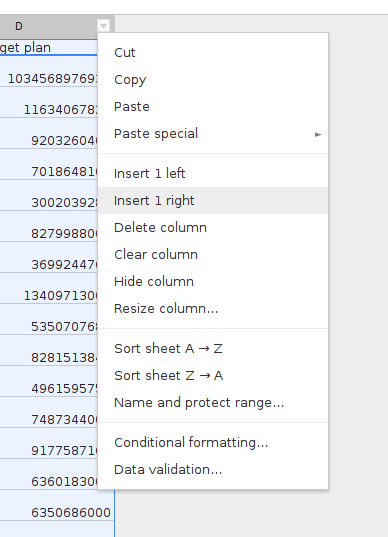
• This gives us a column to work in

• We’ll not give a title right now – we’ll name it when we’re done (since there will be many changes in it)

• Note: If combining formulas seems too confusing for you, we could achieve the same result by having multiple columns with intermediate results. For example, we might create a column AA that contains the output from one formula applied to another column (setting column AA to =THISFORMULA(C), perhaps) and then take the contents of that column and feed it into another formula in another column (such as column BB, setting it to +THATFORMULA(AA) for example).

• The formula we’re going to use is SUBSTITUTE – if you start typing ‘=SUBSTITUTE’ in the spreadsheet, you’ll see the help. three parameters are mandatory: the text we’re working on, what we’re searching and what we want to substitute it with. We’re searching for “MC” and want to substitute it with “City”

• So the formula we’ll be using looks like =SUBSTITUTE(C2,"MC",City") :

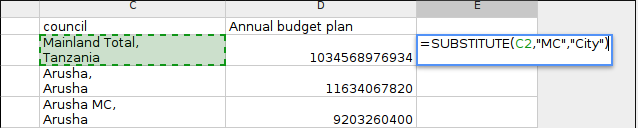
What happens is here is the following: if in the cell C2, there is the word “MC”, replace it with the word “City”.

Note the order: =SUBSTITUTE(CELL,"FROM THIS","TO THAT"). (Some programming languages may refer to this as replace). If you try this out you’ll see how it works: nothing will change with cells like C2, where the word MC is not present, but two cells below, “Arusha MC, Arusha”, as found in cell C4, become Arusha City, Arusha.

• But we want to go further, because we also want to substitute “TC” with “Town”. We could keep creating new columns, passing the results created in one column into a formula in the next that works on those results. Or we can place one function inside another, passing the results from the “inner” one directly into the function that wraps it, as in this example: =SUBSTITUTE(SUBSTITUTE(C2,"MC","City"),"TC","Town").

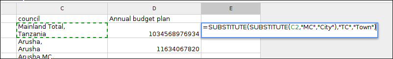
What happens here is the following:

if in the cell C2, there is the word “MC”, replace it with the word “City”, then if in the resulting text there is the word “TC”, replace it with the word Town. Or, using the formula format: SUBSTITUTE(DATA,"TC","Town") where DATA corresponds to SUBSTITUTE(C2,"MC","City")

• So this will do our town and city substitutions, but now we need to work out how to match the combined council and region names. There are two ways we can do this: either, in the census sheet, we could combine the two columns representing the council and a the region into a single column that replicates the formatting of the budget sheet; or in the budget sheet, we could split out the combined council/region names into two columns to match the formatting used in the census sheet. Generally, splitting data is more useful because it provides us with more information, or at least, access to the same information but in a more granular way.

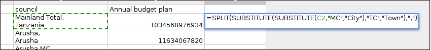
• Luckily Google spreadsheets allows us to easily split columns (other spreadsheet programs allow this too, but tend to be more complicated). It offers a formula called SPLIT, which asks for a text and what to split the text by (in our case “,”)

• Once again, we could create a new column that applies this operation to a column that contains the results of our substitutions, or we can pass that data directly into it. Following that second approach, our formula now looks like this: =SPLIT(DATA,”,”). Which is to say, this: =SPLIT(SUBSTITUTE(SUBSTITUTE(C2,"MC","City"),"TC","Town"),",").

• Now the magic moment has come to press Enter and see whether it does what we want.

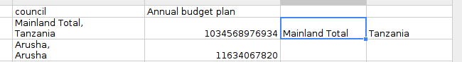
• Looks good, let’s apply this to all rows by double clicking on the small blue square bottom right.

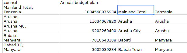
• Fantastic, we have now the council names in the same format as in the other sheet – and you learned how to stack formulas to do even more complicated things.

All you need to do now is to think of a way to appropriately name the columns.

Joining Sheets

Next we need to get information from one sheet to the next sheet – get the population counts into the budget sheet to be able to calculate spending per citizen.

To do this we’ll use a new formula called VLOOKUP – VLOOKUP helps you retrieve related information from other sheets and associate this information with the right row.

Walkthrough: Joining sheets with VLOOKUP

• Create a new column right of the last column we’ve created

• Next, let’s write our formula: VLOOKUP wants 4 parameters (the last one is most often 0)

• The first parameter is the term we’re searching. This is a term present in both sheets, which is used as a reference by the formula to retrieve the correct values. In our case this term is the name of the council.

Note: We assume here that the same council name does not appear in more than one region. In the general case, you should be really careful about assumptions you make when matching items, which is why we prefer matching on proper, unique identifiers. The longer the matched item (for example, council + region) the more likely the item is to be unique. However, the longer the matched item, the harder it is to get an exact match. For example, “City, Region” would not match “City , Region” because the second element contains a space before the comma that does not in the first.

• The second parameter is a selection of the cell range we want to bring matched data in from, as well as the range of values we want to import. In our case, this corresponds to the columns C and D of the second sheet: the first index column is the column that has to contain the term we’re searching for, the rest of the columns represent data we could import data from.

• The third parameter is the column to return from the range specified in the second parameter, counting from the first (index) column which we refer to as column number 1; in our case, we want to pull data in from column 2, the second column.

• The last parameter we set to the value 0 to indicate that we only want to match items on an exact match.

• Our formula looks like this: VLOOKUP(E2,Sheet2!C:D,2,0)

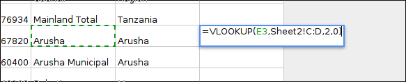
• If you press enter, you’ll see the value is filled into the cell – let’s extend this to all cells by filling downs as we did before, by double clicking on the small blue square in the lower right hand corner of the cell.

• Notice that there may be some cells containing unknown #N/A values when you scroll down – these are the fields that could not be matched. You can compare the first and second sheet to find out what’s wrong.

• Now we can calculate the Spending per person by dividing the budget column by the population column.

Summary

Let’s quickly recap on what you’ve learned so far: you’ve seen how you can combine several Google Spreadsheets formulas by placing on inside the other, in this case by placing one SUBSTITUTE formula inside another, and then both of this inside a SPLIT formula. The innermost formula runs first and then passes its results to the next formula up that contains it. We could alternatively have used each formula within a new column in turn, with the next formula in the chain working on data from the previous column, but taking such an approach may clutter our spreadsheet needlessly. (Such an approach does, however, show your working at each step, we can be useful if an error ever crops in to your spreadsheet!)

You also learned how to use the VLOOKUP() formula to combine data from two separate sheets that share a column column. It did not matter that the order of the rows was different in the two sheets – the VLOOKUP formula was able to take each cell value from the column in the first sheet and then look up the same value in the second. The value the was returned was the value of a the cell in a specified column from the matched row in the second sheet.

Extension Activity – Querying a Data Set

As well as using spreadsheets as a tool to manipulate data, for example, by splitting columns or combining data from different sheets into a single sheet, we can also use Google spreadsheets to run simple database like queries over the data set.

The School of Data course (An Introduction to SQL Databases for Analysing Data) gives a more complete introduction to making queries of data in a simple database using the SQL query language, but it’s worth noting that Google spreadsheets can also run queries written using a very similar language.

Queries are written using a query that is contained within a QUERY formula.

• Create a new sheet and in the first cell enter an empty query that simply pulls in the the data from the first sheet: =QUERY(‘Sheet2’!A:G)

• From within this cell range we can then start to run particular queries (refer to the School of Data course on simple SQL for more ideas). For example, we can just pull back data from specified columns: =QUERY('Sheet2'!A:G, "SELECT A, C, D")

• If we want to find a council in a particular region, we can search by region, for example: =QUERY(‘Sheet2’!A:G, “SELECT A, C, D WHERE A=’Kilimanjaro'”)

• We could refine the query even further, for example by finding councils in a particular region where the total population is greater than or equal to a particular amount: =QUERY('Sheet2'!A:G, "SELECT A, C, D WHERE A='Tanga' AND D>=200000")

• As the examples in the SQL course show, we can summarise data by group, such as counting how many councils are in each region: =QUERY('Sheet2'!A:G, "SELECT A, COUNT(C) GROUP BY A")

• We might also try to find the total population in a region: =QUERY('Sheet2'!A:G, "SELECT A, SUM(D) GROUP BY A") However, when doing this sort of calculation, we need to check that a total amount for the region is not specified along with the values for each council – or we would be double counting!

For a full reference of query language commands, see the Google Visualiastion API Query Language Reference documentation. For an introduction to writing SQL like queries in general, see the School of Data course An Introduction to SQL Databases for Analysing Data.