Spreadsheet Formulae

This tutorial uses Google spreadsheets to analyse data. Other spreadsheet programs work in a similar way – play around and see how they differ.

There is sample data for this tutorial here: http://bit.ly/Y11xkF

A quick introduction to common spreadsheet symbols

Now that you have a sense of how spreadsheet formula work, here’s a quick introduction to some of the most common formula symbols that you are likely to come across.

The symbols

These are all ‘basic maths functions’ – the kind of things you would find on a simple calculator.

=: Tells your spreadsheet that you are writing a formula. This is the first thing that should go in your formula cell. (NOTE: A spreadsheet assumes that everything that begins with an ‘=’ is a formula… so be careful how you use it!)
+: Add
-: Subtract
*: Multiply (this would be ‘x’ on a calculator)
/: Divide (this would be ‘÷’ on a calculator)

Tip: Get your symbols in the right order

It is worth remembering that basic maths rules about the order of functions apply. For example, the formula =3+5*2 will give you 13, NOT 16. If you’re not sure why or can’t quite remember the rules, check out this basic introduction. If you want to change the order of function you’ll need parentheses: Formulas inside parentheses will be evaluated before any other formula. If you want the formula above to result in 16 you’ll need to type: =(3+5)*2

Have a go at using these formula in the ‘play sheet’ of your spreadsheet until you feel comfortable with them. You should find that they work pretty much as you would expect them to.

What if you wanted to add more numbers? You could always add them manually using + or you could use SUM a formula to sum up all the values in the given range. Let’s try to calculate how many apples, plums and total fruit we sold during the week: Go to cell B7 and type =SUM(B2:B6) this will add the numbers of apples.

Walkthrough: Using spreadsheets to add up values.

Let’s calculate the total of fruits sold.

Get the example data and create a copy.

To start, move to the first row.

Each formula in a spreadsheet starts with =

Enter = and select the first cell you want to add. Notice how the cell reference appears in the formula?

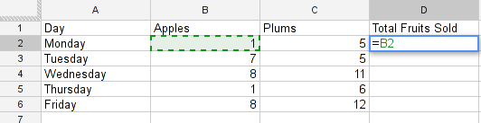
now type + and select the second cell you want to add

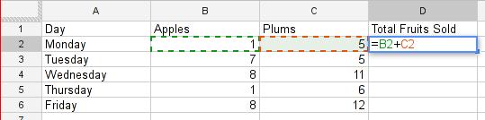
Press Enter or tab .

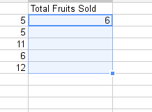
The formula disappears and is replaced by the value.

Try changing the number in one of the original cells (apples or plums) you should see the value in total update automatically.

You can type each formula individually, but it also possible to cut and paste or drag formulas across a range of cells.

Copy the formula you have just written (using ctrl + c ) and paste it into the cell below (using ctrl + v ), you will get the sum of the two numbers on the row below.

Alternatively click on the lower right corner of the cell (the blue square), and drag the formula down to the bottom of the column. Watch the ‘total’ column update. Feels like magic!

Walkthrough: Using a spreadsheet to subtract values.

Take a look at the above example – it’s exactly the same, apart from you use a - instead of a +. Easy! Find the difference between the two columns in the example above.

Walkthrough: Multiplication and Division

Math recap: If you have a percentage and the value it is associated with you can calculate the value of the percentage. e.q. let’s say 25% of people in a town of 1000 inhabitants are below 15 years. You can calculate the number of inhabitants by using the following formula:

number of inhabitants in a town x (25 ÷ 100)

In a spreadsheet – the above answer expressed simply by:

=25*1000/100

(For more thorough explanation of percentages check out BBC Skillswise )

Now for a more complicated example:

Let’s go back to our World Bank dataset. If you haven’t done the previous tutorials or lost the file: download it here .

In our original data, we have three columns related to health expenditure; ‘health expenditure (private)’, ‘health expenditure (public)’ and ‘health expenditure (total)’. So we’ll need to add three new columns to the right of the spreadsheet to do your calculations. Give them each a heading; perhaps ‘health expenditure (private) in USD’ etc.

In the original data, public, private and total healthcare expenditure is expressed as a % of GDP. The GDP is already given in USD. To work out the expenditure in USD from these two facts is just one step. We want to calculate how much money (in USD) is spent on healthcare per country and year.

Let’s start by looking at the very first complete row (NB: spot the gap! we don’t have the data for Afghanistan’s GDP in 2000. Just be aware of this for now (we will talk in more detail about gaps in data later). The first complete row is Afghanistan in 2001.

In 2001, Afghanistan’s GDP was $2,461,666,315. Their private healthcare expenditure was 6.009337744 % of this. So the calculation you need to do is

2461666315 * 6.009337744 / 100

With a spreadsheet formula, we don’t have to worry about all the numbers – you just need to enter the cells. So the formula you are going to need is: =E3*H3/100 (where cell E3 contains Afghanistan’s GDP in 2001, and cell H3 contains private health expenditure in Afghanistan in 2001).

Drag this formula all the way down the column and hey presto! You should have calculated the private health expenditure in USD for every country for the past 10 years. Much quicker than doing all the sums yourself!

Walkthrough: Copying formulae sideways

In the same way as we could drag the formula down the column and the spreadsheet recognised the pattern and chose the correct cells, we can also drag the formula sideways to the new columns (public health expenditure in USD and total health expenditure in USD). So, if we want BUT we need to make one minor adjustment.

Still using the World Bank Data, try just dragging a cell formula across. Can you see the problem? The spreadsheet automatically moves all the cells its looking at one column to the right. So whereas before we had:

=E3*H3/100

we now have

=F3*I3/100

…but GDP is still in column E, so this formula is not the one we want.

To ‘fix’ a column or row, all you need to do is add ‘$’ in front of the section you want to fix. So, if you adapt your original formula to…

=$E3*H3/100

…you should be able to drag it over to the right without any problems.

Tip:

It can be a little confusing getting used to the $ command at first. If this is the first time you’ve come across it, we suggest you spend some time playing around and seeing what it can do. Go back to your ‘play’ spreadsheet, make up some numbers, and experiment! Try for example =$B2*C2 vs =B$2*C2, drag it around, and see what difference that makes. The best way to get comfortable with formulae is to use them!

So now, with one simple formula, you can calculate the actual expenditure of public, private and public+private healthcare, in every country, for the past ten years. Spreadsheets are pretty powerful things.

Walkthrough: Minimum and Maximum Values

One thing that is very interesting to us when working with data is the maximum and minimum values of each of the columns we have. This will help us understand if the values are close together or far apart. Let’s do this!

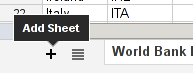
Open a new sheet. Do so by clicking the “+” in the lower left corner

Leave the first column in the first row blank, in the second column enter = to tell the spreadsheet you will be using a formula.

Switch back to the sheet with your World Bank dataset.

Select the first column that has numerical data on the sheet where your data lives.

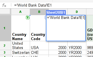
Press enter and you will see the name in the first sheet: magic. Why do we do it like this and not simply copy and paste? This will automatically change the headings if you change your headings (e.q. you move columns around or rename things).

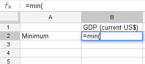
Now the first column is going to be what you calculate: type Minimum in the second row first column (A2) for the minimum value.

In the cell right next to it type =MIN( (MIN is the formula for minimum)

Go back to the other sheet to select the first column with numerical data – to select the whole column click on the grey area with the column letter.

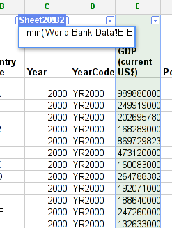
Close the brackets by typing ).

You should now see the minimum value in that field.

Now do the same for Maximum in the third row. Once you are done, just mark the three values in the second row (the formula for maximum is =max() )

See the blue square in the right lower corner? Grab it and pull it right. Release it and if you still not have all columns, carry on until you have all values.

This way you created a table with the minima and maxima of each of the columns.

Walkthrough: Dealing with empty cells

Did you notice some of the minimum values are 0? Do you really believe there are countries not spending money on healthcare? There aren’t (well, probably). The zeroes are because there are empty cells. Properly handling missing values is an important step in data cleaning and analysis – hardly ever are large datasets complete and you have to find a strategy to deal with missing parts.

In this walkthrough we will create a complex formula. We will do so with an iterative process – this means one little formula at the time. If you follow us through you’ll notice you can create quite complex formulas and results simply step by step.

To deal with empty cells we have to fix parts of our calculation formulas in the World Bank datasheet

To start – create a mock spreadsheet to play with data. Copy the first few rows of the World Bank dataset into it so you’ll have a start. To validate our formulas try to remove values in some of the rows.

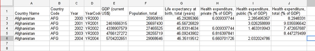
We got a missing problem right in the first value: Afghanistan’s GDP is missing for the year 2000.

Think about our goal. What we want to achieve: if either of the values we are multiplying (in this case, GDP or health expenditure) is not a number (probably because the value is missing), we don’t want to display the total.

To put it another way: only if a value for both GDP and healthcare expenditure is present should the spreadsheet carry out the calculation; otherwise it should leave the cell blank.

The formula to express this condition is ‘IF’. (You can find an overview on formulas like this on the google doc help.)

The formula asks us to fill out the three things: (1) Condition, (2) value if the condition is true, (3) value if the condition is false.

=IF(Condition, Value if condition is true, Value if condition is false)

In our case we know parts (2) and (3). (2) is the formula we used above this is the calculation we want to carry out if both values are present in the spreadsheet.

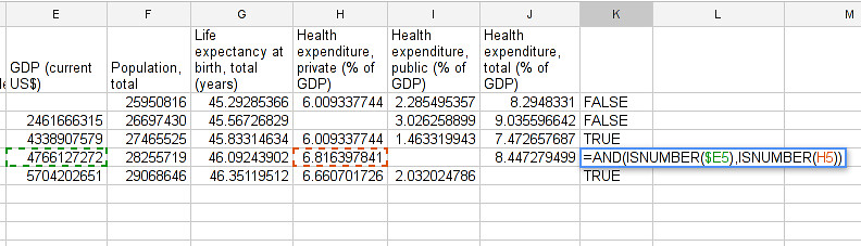
=IF(Condition, $E3*H3/100, Value if condition is false)

(3) is a blank – if the numbers aren’t there, we don’t want to display anything, so we fill in that value with nothing at all.

=IF(Condition, $E3*H3/100,)

So now we just need to work out (1), the condition.

=IF(Condition, $E3*G3/100,)

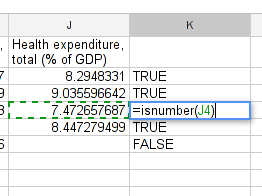
Remember that we want the condition to be that BOTH the GDP and healthcare expenditure values are a number. The formula to see whether a cell is a number is: ISNUMBER.

This is another one of those little formulas that you should try playing with! If you type =ISNUMBER(F2) and F2 is an empty field, it will say FALSE. If there is a number it will say TRUE. Handy isn’t it?

We want a formula that will only be calculated if both GDP and healthcare expenditure are actual numbers.

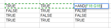
We need to combine the results of both ISNUMBER(GDP) and ISNUMBER(healthcare expenditure) together. The formula to do so is AND. This will simply say TRUE if both of them are TRUE (i.e. both of them numbers) or FALSE if either one or both of them is FALSE.

Which is exactly what we need. So our condition will be:

AND(ISNUMBER(gdp),ISNUMBER(healthcare expenditure))

or, to use our cells from before

AND(ISNUMBER($E3),ISNUMBER(H3))

Phew! So now we can put parts (1), (2) and (3) from above all together in one big formula, using ‘IF’

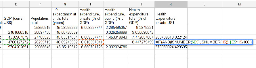
=IF(Condition, $E2*H2/100,)

=IF(AND(ISNUMBER($E2),ISNUMBER(H2)),$E2*H2/100,)

Try it out: enter it to the first row of the first column of the calculation and paste it to all the other places. It should leave the cells empty.

If you look at the data you will quickly find out that countries with higher number of people spend more on healthcare than countries with lower number of people. Intuitive isn’t it. So how to compare the countries more directly? Break it down to healthcare expenditure per person!. This step is called normalization and is a step often done when comparing different entities – such as countries etc.

Any questions? Got stuck? Ask School of Data!

Last updated on Sep 02, 2013.