Using Excel to do data journalism
This is a report from the School of Data Journalism organised by Open Knowledge,European Journalism Centre, and International Journalism Festival. The session was led by Steve Doig, Knight Chair in Journalism, specializing in computer-assisted reporting — the use of computers and social science techniques to help journalists do their jobs better.
You can download Steve’s presentation and the data used in this tutorial here.
Microsoft Excel is a powerful tool that will handle most tasks that are useful for a journalist who needs to analyze data to discover interesting patterns. These tasks include:
- Sorting
- Filtering
- Using math and text functions
- Pivot tables
#Introduction to Excel
Excel will handle large amounts of data that is organized in table form, with rows and columns. The columns (which are labeled A, B, C…) list the variables (like Name, Age, Number of Crimes, etc.) Typically, the first row holds the names of the variables. The rest of the rows are for the individual records or cases being analyzed. Each cell (like A1) holds a piece of data.
Modern versions of Excel will hold as many as 1,048,576 records with as many as 16,384 variables! An Excel spreadsheet also will hold multiple tables on separate sheets, which are tabbed on the bottom of the page.
#Sorting
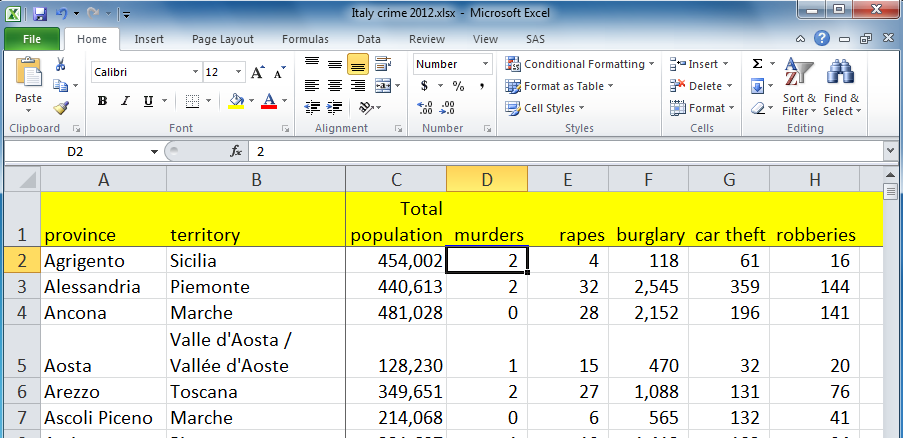
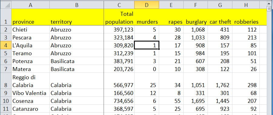
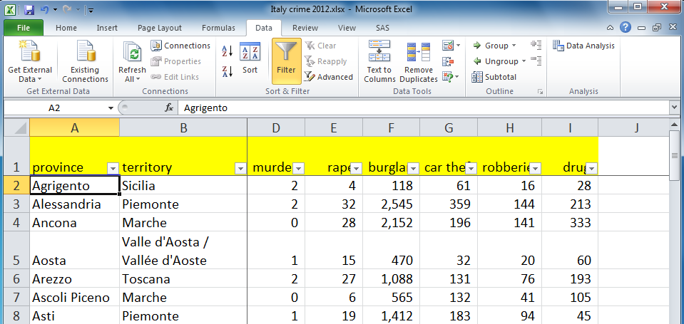
One of the most useful abilities of Excel is to sort the data into a more revealing order. Too often, we are given lists that are in alphabetical order, which is useful only for finding a particular record in a long list. In journalism, we usually are more interested in extremes: The most, the least, the biggest, the smallest, the best, the worst. Consider the data used in this workshop, a list of the provinces of Italy showing the number of various kinds of crimes reported during a recent year. Here is how it looks sorted in alphabetical order of province name:

Far more interesting would be to sort it in descending order of the total number of murders, with the most violent city at the top of the list:
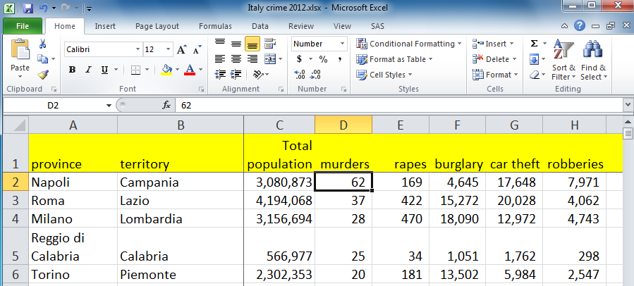
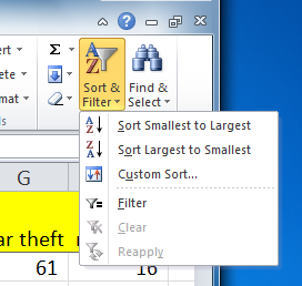
There are two methods of sorting. The first method is quick and can be used for sorting by a single variable. Put the cursor in the column you wish to sort by (“Murders” in this case) and then click the A-Z icon:
You’ll get a window that looks like this:
Sort in whichever order you want. But beware! Put the cursor in the column, but DO NOT select the column letter (D, in this case) and then sort. Consider the example below:
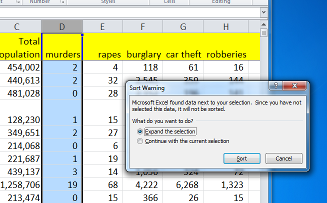
You will get that warning message, but don’t choose “Continue with the current selection”. That will sort ONLY the data in that column, thereby disordering your data! The other method of sorting is for when you want to sort by more than one variable. For instance, suppose we wish to sort the crime data first by Territory in alphabetical order, but then by “Murders” in descending order within each Territory. To do that, go to the toolbar, click on the “Data” tab and then the “Sort” icon, and then choose the variables by which you wish to sort. (Click “Add level” to add new levels.) Then click “OK”.
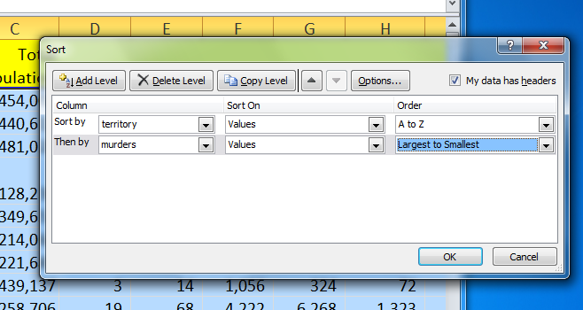
The result will be this:
Filtering
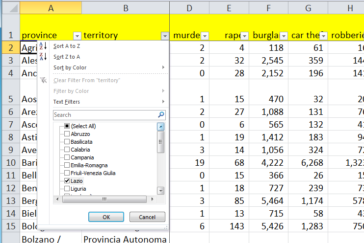
Sometimes you want to examine only particular records from a large collection of data. For that, you can use Excel’s Filter tool. On the toolbar, go to the “Data” tab, then click “Filter”. Small buttons will appear at the top of each column:
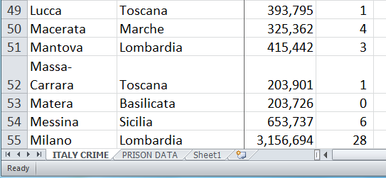
Suppose we wish to see only the records from the Territory of Lazio. Click on the button on the Territory column, uncheck the “Select All” box, and then choose Lazio from the list, like this:
This is the result:
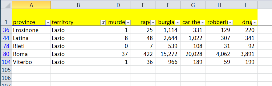
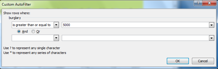
Notice that you now are seeing only rows 36, 44, 78, 80 and 104. The rest are still there, but hidden. More complicated filters are possible. For instance, suppose you wish to see only records in which “Burglaries” is greater than or equal to 5,000 AND car thefts is less than 2,000. You start by filtering Burglaries like this:
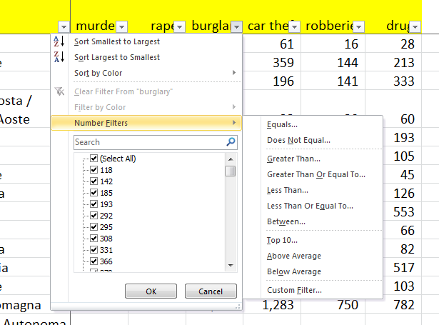
then this…
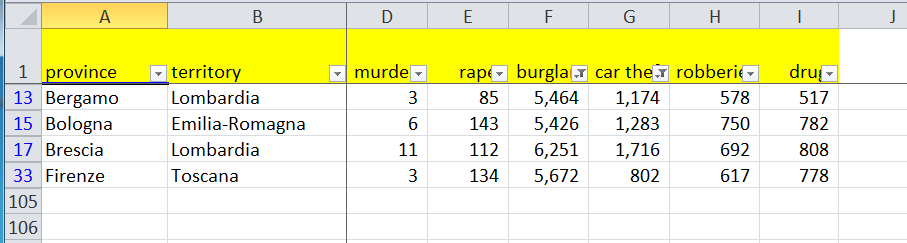
Do the same for Car Thefts, and you get this:
Functions
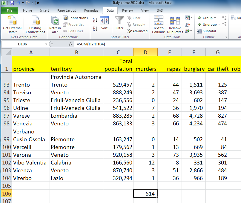
Excel has many built-in functions useful for performing math calculations and working with dates and text. For instance, assume that we wish to calculate the total number of murders in all the provinces. To do this, we would go to the bottom of Column D, skip a row, and then enter this formula in Cell D106: =SUM(D2:D104). The equals sign (=) is necessary for all functions. The colon (:) means “all the numbers from Cell D2 to Cell D104”. After you hit Enter, the result is this:
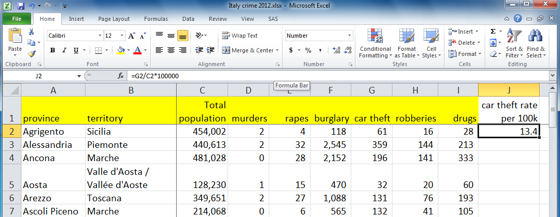
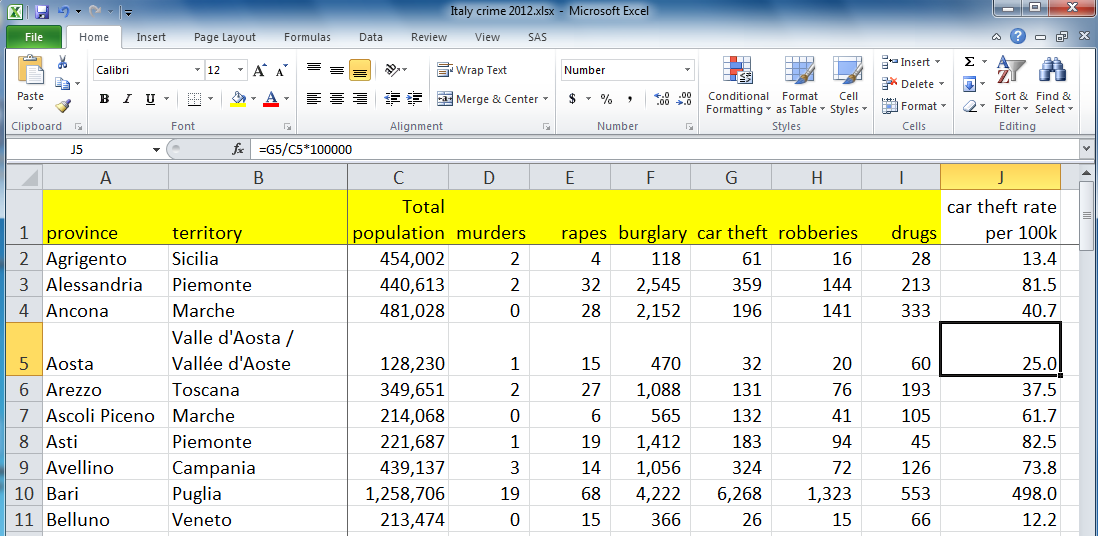
(The reason for skipping a row is to separate the sum from the main table so that the table can be sorted without pulling the sum into the table during the sorting operation. This way the sum will stay at the bottom of the column. Often you will want to do a calculation on each row of your data table. For instance, you might want to calculate the auto theft rate (the number of cars stolen per 100,000 population), which would let you compare the auto theft problem in cities of different sizes. To do this, we would create a new variable called “Car Theft Rate per 100k” in Column J, the first empty column. Then, in Cell J2, we would enter this formula: =(G2/C2)*100000. This divides the stolen cars by the population, then multiplies the result by 100,000. (Notice that there are no spaces and no thousands separators used in the formula.) Here is the result:
You can format your numbers using various choices in this box under the “Home” tab: 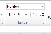 It would be very tedious to repeat writing that calculation in each of 103 rows of data. Happily, Excel has a way to rapidly copy a formula down a column of cells. To do that, you careful move the cursor (normally a big fat white cross) to the dot on the bottom right corner of the cell containing the formula. When it is in the right spot, the cursor will change to a small black cross. At that point, you can double-click and the formula will copy down the column until it reaches a blank cell in the column to the left. This would be the result:
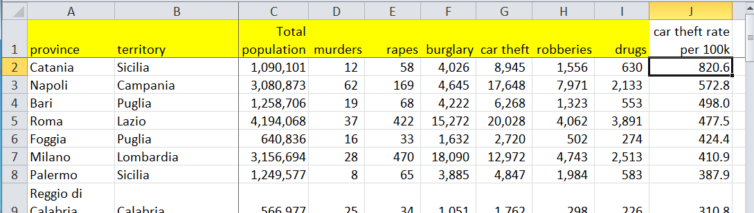
Notice that the formula changes for each row, so that the Row 5 formula is =G5/C5*100000, and so on. That’s what makes Excel so powerful — the ability to change formulas as you copy down or across. Now, if we sort by Car Theft Rate in descending order, we see the cities with the worst auto theft problems:
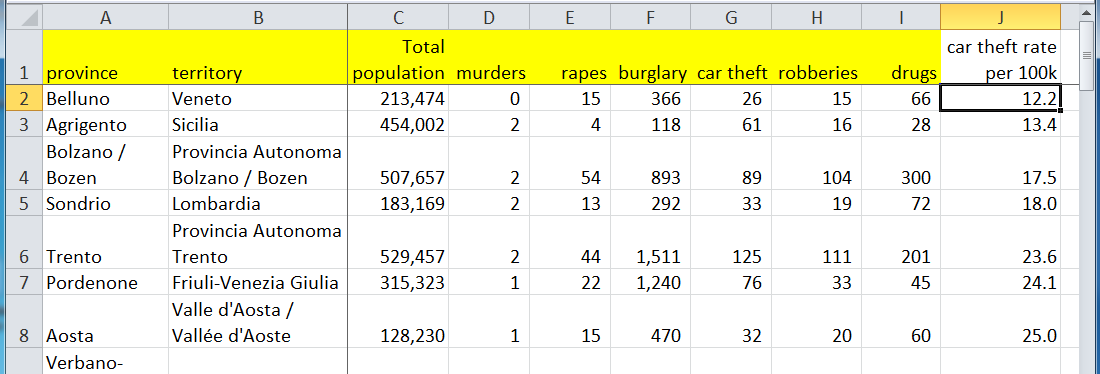
and sorting in ascending order, the least crime:
Here are some other useful Excel functions that can be used in similar ways:
(You can add, subtract, multiply or divide by using the symbols + – * and /)
- =AVERAGE – calculates the arithmetic mean of a column or row of numbers
- =MEDIAN – finds the middle value of a column or row of numbers
- =COUNT – tells you how many items there are in a column or row
- =MAX – tells you the largest value in a column or row
- =MIN – tells you the smallest value in a column or row
There are also a variety of text functions that can join and cut apart text strings. For instance:
If “Steve” is in Cell B2 and “Doig” is in Cell C2, then =B2&” “&C2 will produce “Steve Doig”. And =C2&”, “&B2 will produce “Doig, Steve”. Other text functions include:
- =SEARCH – this will find the start of a desired string of text in a larger string.
- =LEN – this will tell you how many characters are in a text string.
- =LEFT – this will extract however many characters you specify starting from the left.
- =RIGHT — this will extract characters starting from the right.
- =MID — this will start extract where you tell it to start, and get as many characters as you specify.
You can also do date arithmetic, such as calculating the number of days or years between two dates, or hours, minutes and/or seconds between two times. For instance, to calculate on April 24, 2014, the age in years of someone whose birth date is in cell B2, you could use this formula: =(DATE(2014,4,24)-B2)/365.25. The first part of the formula calculates the number of days between the two dates, then that is divided by 365.25 (the .25 accounts for leap years) to produce the years. Another useful date function is =WEEKDAY, which will tell you on which day of the week a chosen date falls. For instance =WEEKDAY(DATE(1948,4,21)) returns a 4, which means I was born on a Wednesday.
Pivot Tables
One of Excel’s best tricks is the ability to summarize data that is in categories. The tool that does this is called a pivot table, which creates an interactive cross-tabulation of the data by category. To create a pivot table, every column of your data must have a variable label; in fact, it is always good practice to put in a variable label as soon as you insert or add a new column.
First, you make sure your cursor is on some cell in the table. Then go to the tool bar, click on the “Insert” tab, and then click on the “Pivot Table” icon. A window will pop up that looks like this:
Excel offers well over 200 functions in a variety of categories beyond just math, dates and text: Financial, engineering, database, logical, statistical, etc. But it is unlikely that you will need to be familiar with more than a dozen or so functions, unless you are a journalist with a very specialized beat such as economics.
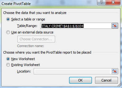
Normally, all you need to do is hit “OK”. This will open a new sheet that looks like this:
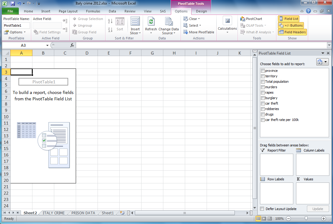
To build a pivot table, you should visualize the piece of paper that would answer your question. Our example data shows 103 provinces in the 20 Territories of Italy. Imagine that you wanted to know the total number of murders in each Territorio. The piece of paper that would answer that question would list each Territory, with the total number of murders next to each name.
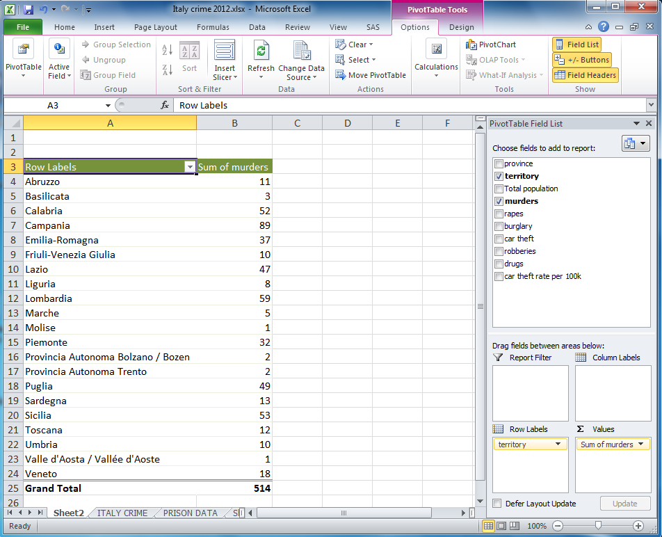
To build this pivot table, we would use the mouse to pick up “Territory” from the list of variables in the floating box to the right, and place it in the “Row Labels” box below. We would then take the “Murders” variable and put it in the “Values” box. This would be the result:
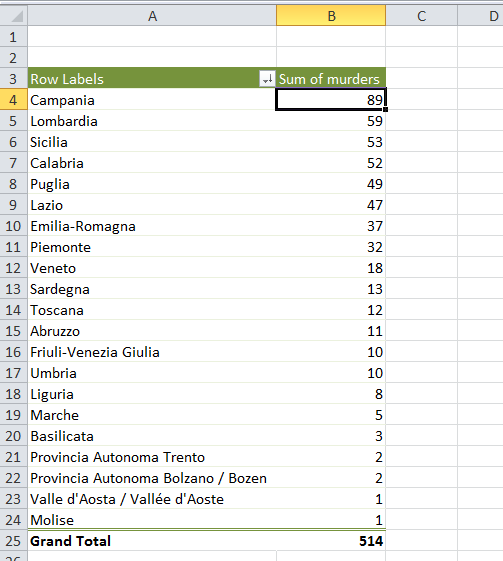
If you click the cursor into the “Total” Column and hit the Z-A button to sort, you will get this:
It is possible to make very complicated pivot tables, with multiple subtotals. But I recommend making a new pivot table for each question you want to answer; several simple tables are easier to understand than one very complicated table that tries to answer many questions at once.
The little black down-arrow button on the “Values” variable opens up a box that will let you make a variety of other choices about how to summarize and display the result. Click on “Value Field Settings” and you get this:

Other Excel Tips
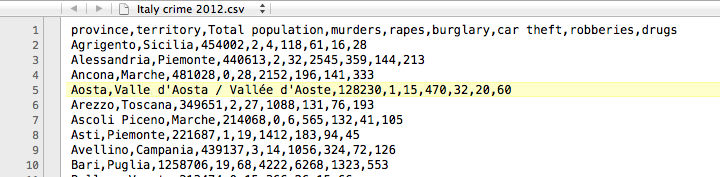
Excel will import data that comes in a variety of formats other than the native *.xls or *.xlsx that Excel uses. For instance, Excel can readily import text files in which the data columns are separated by commas, tabs, or other characters, like this:
If you find a web page with data in table format (rows and columns), Excel can open it as a spreadsheet. Copy the table and then paste it into Excel; very often it will flow properly into the correct columns.
Finding Data
Government agencies are starting to make some of their data available in Excel or other formats. For example, ISTAT.IT has very comprehensive data about Italian demographics, economy, crime, etc. Many of their tables can be downloaded directly as Excel files.
One trick to find interesting data would be to use Google and add these search terms: site:.gov filetype:xls.
![]()