The first online Data Expedition ventured to Flatland to respond to a call for help. Four Teams set out to solve a problem: An epidemic of heaviness. We’re now receiving the teams’ mission reports.

This mission report is the first one in by the “Courteous Clauses” team. Read their full report for a list of their data sources and a detailed breakdown of how they tackled the issue facing them.

The purpose of a data expedition is to encourage teams to explore a topic and learn by working with real-life data. The first data expeditions were offline, and we always expected online to be a lot trickier. We’d like to say a huge congratulations to the groups for their perseverance and we look forward to catching up with a few of the participants at our hangout to learn from their experiences.

Now, over to the Clauses…

Step one: find out who you have in your team and find an angle to approach the problem

Our team, the Courteous Clauses, got off to what seemed a promising start. We made our introductions; set up a Google+ community and a Hackpad; and the programmers/developers/engineers established an organization on GitHub. One team member also put together a survey to get an idea of the mix of people on the team, and it looked like there was a good balance of experience and talent. After some initial confusion over interpretation of Flatland, we formed the general idea that we were to investigate some aspect of obesity in our world so that we might enlighten Flatland with our findings.

Steps two and three: pick a question and find the data

We also found numerous studies on obesity – so numerous that we had trouble deciding on a direction. After soliciting suggestions and taking a vote, we decided to focus on obesity in urban areas, associations with urban density, and comparisons with rural areas. But almost immediately, team members started finding many articles suggesting that this aspect of the obesity problem had already been well covered, for example:
Are obesity rates higher for urban or rural residents?

[Above] Slideshow containing images referenced below

Some team members felt we should find a problem that had not been tackled before – but others felt the pressure of time and the need to have something completed by February 5. The team had already experienced attrition amongst the ranks – and we probably lost a few more team members at this stage.

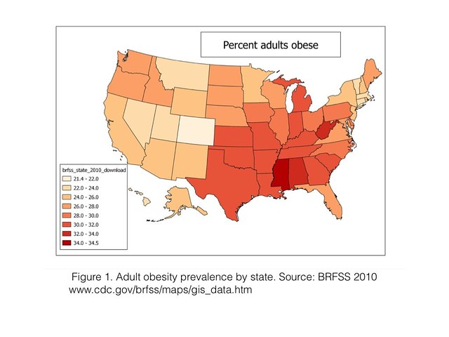
The group started out by collecting amounts of data bout the distribution of obesity in the United States (above) they quickly noted that two neighboring states (Colorado and Kansas) show markedly different percentages of obese males. This struck them interesting and they went on and investigated the issue: they found that obesity percentages are calculated differently for each state based on census data (they are in different census zones) – thus the values might not really be comparable.

A team member pointed out that the neighboring states of Colorado and Kansas present a comparison that might possibly be interesting. Figure 1 shows that Colorado stands out as the least obese state while Kansas ranks much more highly. A comparison of the two states using county-level Behavioral Risk Factor Surveillance Study data is equally striking (Figure 2) – and it was suggested that we might compare the counties of eastern Colorado with those of western Kansas to possibly identify factors that might explain the difference. At this point, a couple of team members did express concern that the “state line effect” might be an artifact of the methods via which the data for these sparsely populated counties were compiled. And their concerns are probably justified, because Figures 3-6 do not suggest any sharp contrasts across the state line. (Data for Figures 2-6 are all from the USDA Food Environment Atlas, 2010).

Poverty levels (Figure 3) appear similar either side of the border, while Figure 4 suggests a somewhat older population in the counties of western Kansas compared with eastern Colorado. Accessibility to large grocery store is more variable in western Kansas (Figure 5), but not necessarily worse overall. Finally, the three counties of western Kansas that stand out in Figure 6 with regard to fast food restaurants just happen to be along the Interstate 70 corridor.

There was one more Colorado-Kansas comparison that was contributed as this was being compiled: Figure 7 compares prevalence of physical inactivity for the border counties of the two states. There is a suggestion of greater prevalence of inactivity on the Kansas side, and were more time available, this would definitely be worth examining further.

Does the right data even exist?

Speaking of non-comparable values – they continued looking into how body mass index might be applied to inhabitants of flatland – realizing that shape matters: some shapes have a similar height but different circumference. Similar humans come in different shapes as well. Someone very muscular might weigh more – but does this make the person obese? Certainly not!

Flatland assesses the weight status of its inhabitants with their own version of our Body Mass Index (BMI). BMI is simply the weight divided by the square of the “height” of a shape measured perpendicularly from one of its sides. In Flatland’s two-dimensional world, the shapes have no measurable thickness – and thus no measurable weight – so we are perhaps to assume that “weight” is simply proportional to area within the shape’s perimeter. This raised immediate concerns about the validity of comparing BMI values across shapes, because the BMI definition only takes into consideration the “height” of the subject. Figure 8 compares BMI of different shapes of the same unit “height.” An equilateral triangle of “height” 1.00 has a BMI of around 0.58. However, the son of this triangle will have a BMI of 1.00. The son of the square, a pentagon, will have a BMI of 0.73. So, a Flatland family of three generations of equal “height” can have a wide range of BMI values on account of geometry alone! (“Height” is placed within quotes because there is no “up” in Flatland and the very suggestion of it could land one in jail!)

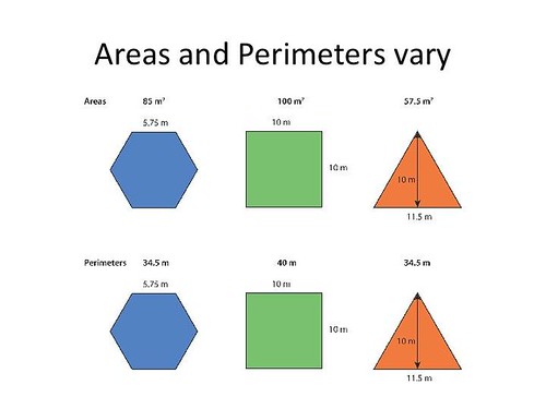
Flatlanders may want to reconsider their formula for BMI as reliable measure of obesity, one that takes into account the different shapes of inhabitants. A hexagon, square, and triangle of the same mass and same geometric height would have the same BMI (Figure 9), even though their different areas and perimeters could suggest that their weight is distributed differently (Figure 10).

They conclude:

In Flatland, and in our own world, a possibility is to determine different cutoff BMI values for different population groups. Or, one could just use some common sense instead of relying on a single number as a measure of weight-related health risk! Unlike Flatlanders, humans are irregular in shape!

An enormous congratulations to the Clauses for their thorough analysis and careful consideration of whether factors were directly comparable. Stay tuned for more mission reports from the front!

Side note: the maps were made in Quantum GIS. More on mapping later in the year from School of Data.